The Problem
When Sensors Fail,
Patients Pay the Price
Cold-chain equipment and lab instruments stream data constantly. Small anomalies go unnoticed until a drug batch is already ruined. BioSentinel catches them as they happen.
01
Cold storage failures
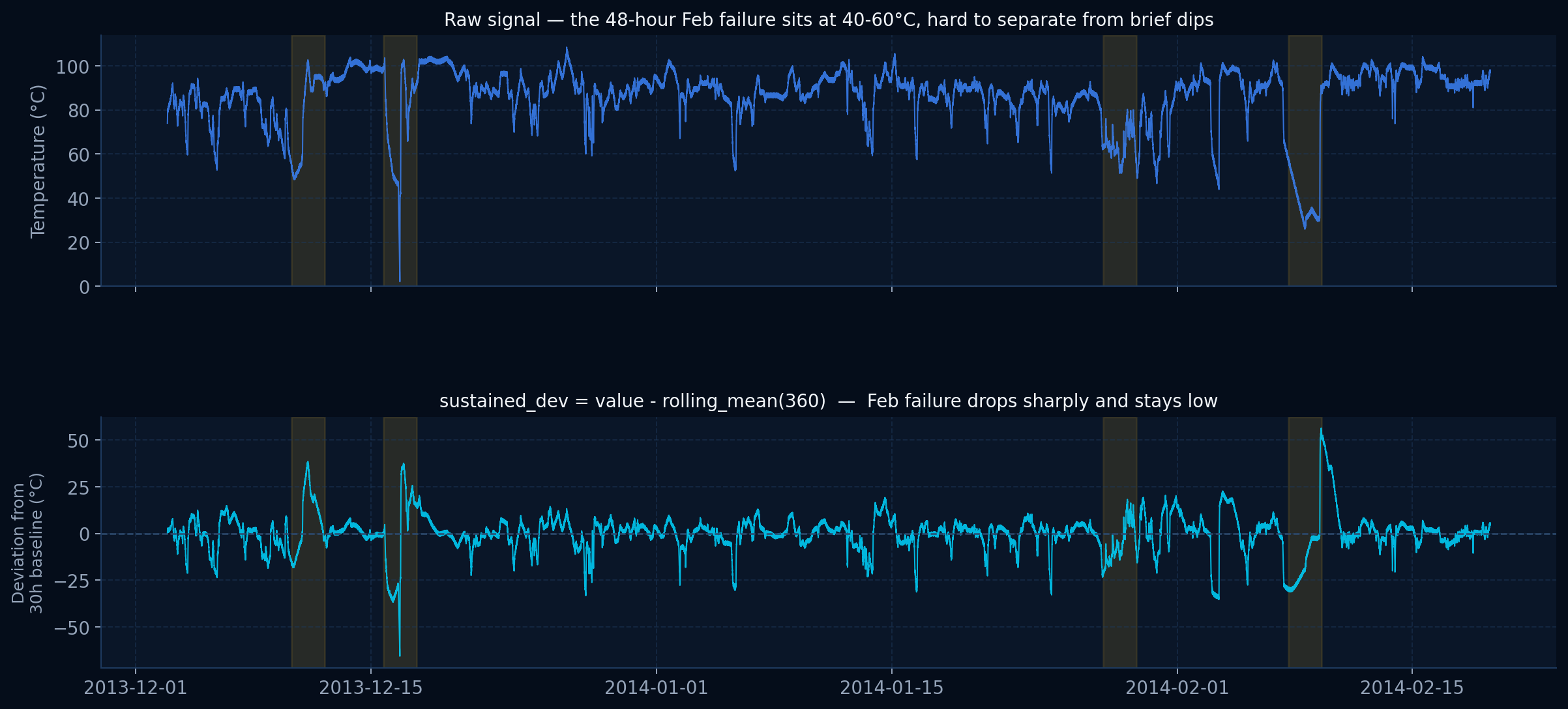
A refrigerator storing vaccines or insulin can fail silently at night. By morning the batch is ruined and patients go without.
02
Sensor tampering
In pharmaceutical settings, tampered or miscalibrated sensors can hide contaminated batches from quality control behind fake-normal readings.
03
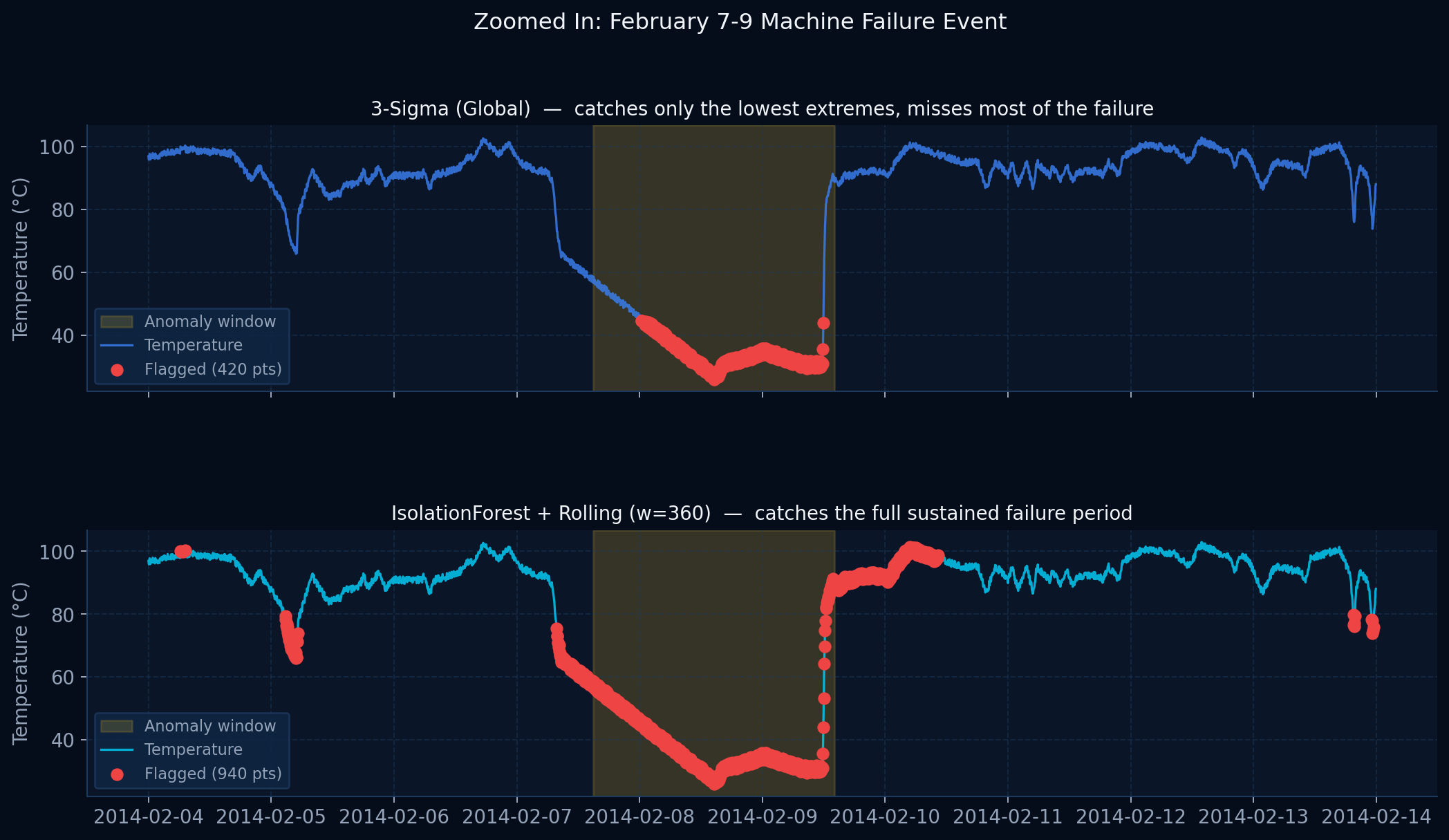
The detection gap
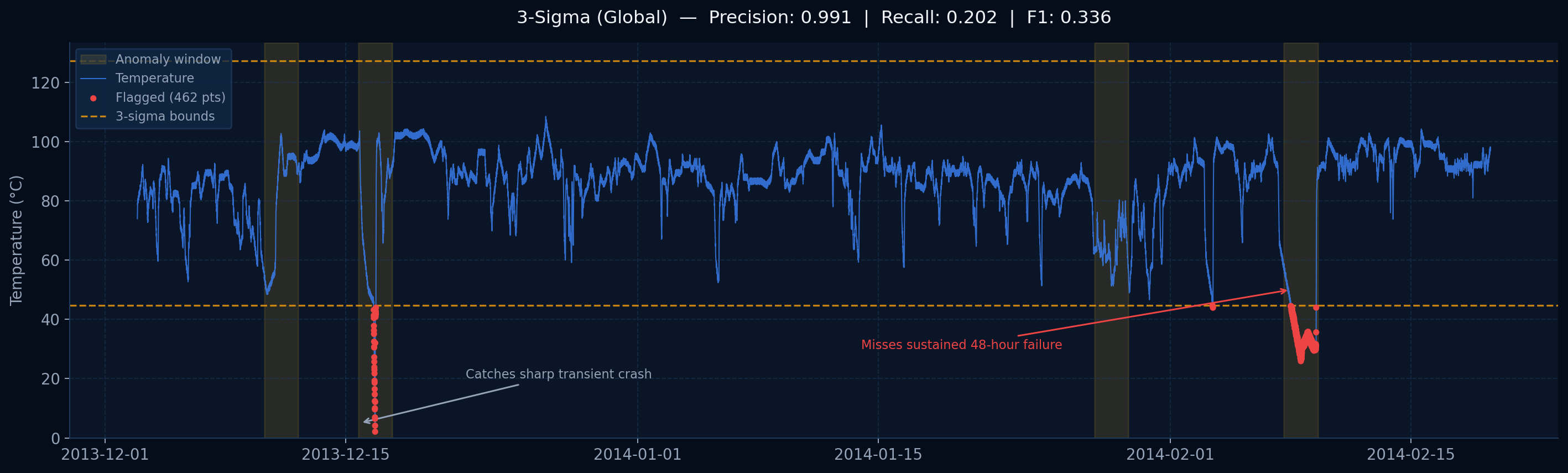
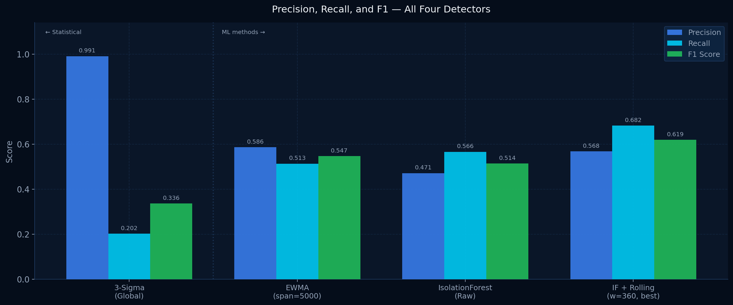
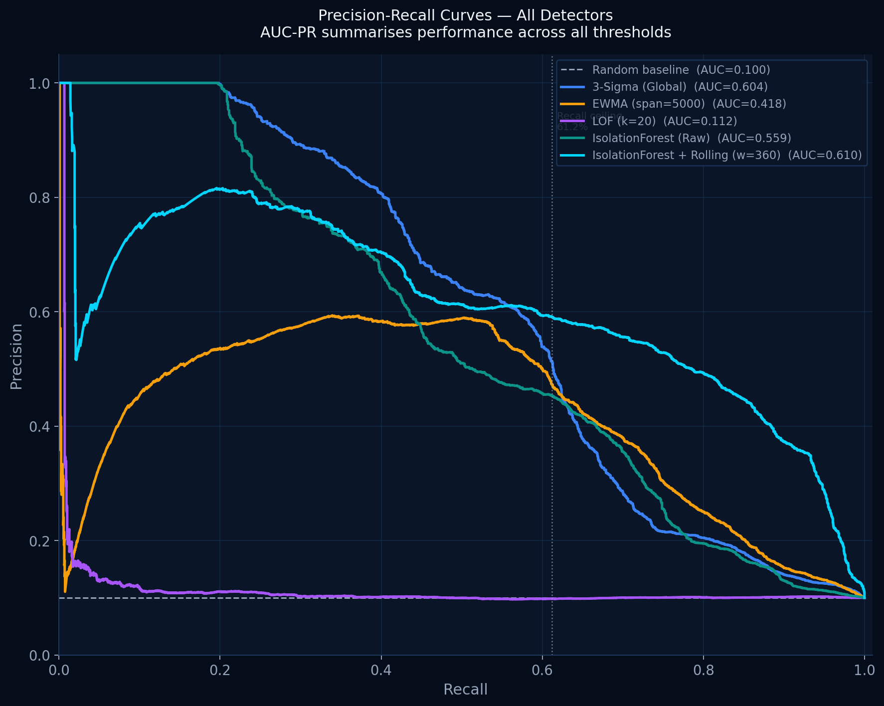
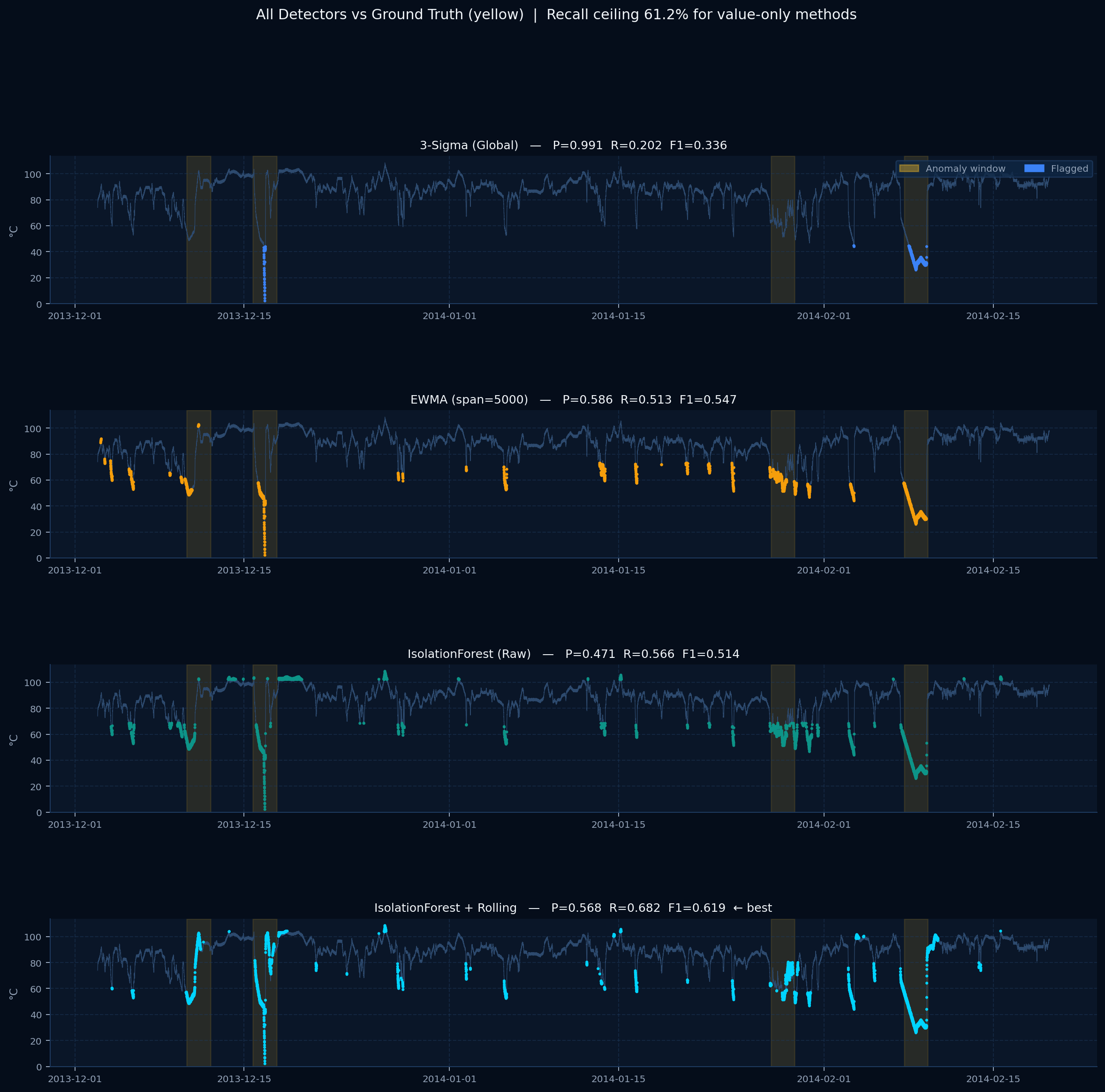
Simple thresholds miss slow sustained failures. Advanced systems exist but are proprietary and unauditable. There is no open baseline anyone can inspect.
04
A security question
Sensor integrity is a security problem, not just a maintenance one. BioSentinel treats it with the same rigor applied to network intrusion detection.
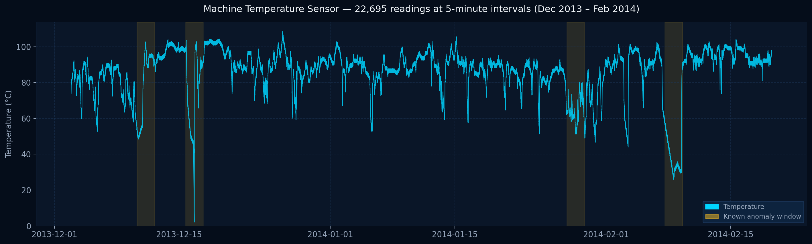
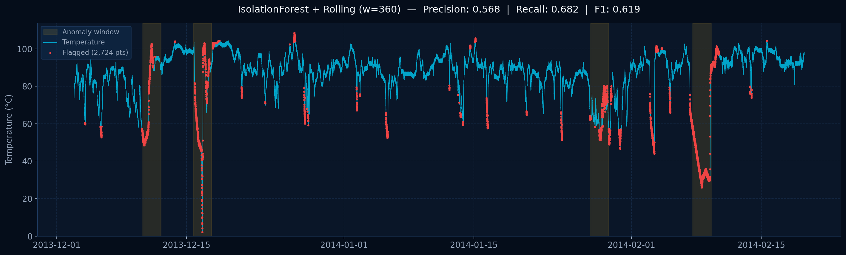
Temperature every 5 minutes
Known anomaly window
NAB machine_temperature_system_failure — Dec 2013 to Feb 2014 — 22,695 rows